Abstract
You will rarely, if ever, have seen an expected-goals figure for a New Zealand domestic game. Where the numbers exist at all they are borrowed, since the models behind them were trained on the elite game and quietly assumed to fit the local game. There is good reason to doubt that they do. In the local game, neither the finishing nor the resistance it meets necessarily matches the professional game the model learned from. If the level is different on both sides of the ball, a model trained on the elite game will misprice a New Zealand shot. The interesting question is by how much, and in which direction. The answer here is a modest lean low, a few goals over the whole test. Using one hundred hand-tagged New Zealand matches, this article builds a hybrid model that learns the shape of shot value from a large elite dataset and corrects the level with local results. Tested on games it never saw, it had the lowest calibration error of the three models compared on every shot, though the differences are too small to separate with this many matches. What follows is how it was built, what the early evidence says, and what it reveals about one club’s season. It is a work in progress, and the more of the local game it sees, the better it gets.
1 The problem with borrowed numbers
Expected goals (xG) is everywhere in the professional game, on broadcasts, in match reports and in conversations about whether a scoreline reflects the chances. The idea is useful. Assign each shot a probability of being scored, then add those probabilities to see what a team created. Yet an xG figure is still hard to find for a New Zealand domestic match.
Commercial data may cover some National League fixtures, but access can be costly and the underlying numbers are rarely available to local clubs and supporters. The grades below are barely covered. For much of the domestic game, the data itself must first be collected, and here that meant tagging matches by hand.
That is the gap this project set out to close, to build a model for New Zealand football that local clubs can use. It also raised a deeper question. If an xG model is trained on elite football and applied here, do its probabilities still fit?
It is tempting to assume an elite model would overvalue local chances because players at this level are less polished finishers. Those players, though, also face defenders and goalkeepers who are just as far from the professional standard. The effect on conversion could go either way. The answer has to come from the shots themselves.
The answer to this conundrum is a hybrid model. A hundred local matches provide too few shots to learn every relationship from scratch. A much larger elite dataset provides a useful starting point for how distance, angle and shot type affect scoring. Local match data then adjusts the resulting probabilities to the level observed here.
The hundredth tagged match is a useful moment to share the work. The database has grown match by match since 2022. It now offers a first test of whether local calibration helps, while leaving room for a much larger sample to settle the details.
2 What expected goals actually is
Expected goals is a probability, not a prediction of a particular result. A shot valued at 0.30 xG is one that the model expects to be scored about 30 times in 100 comparable attempts. The shot itself still produces either a goal or no goal. Figure 1 shows how the estimated chance changes across the pitch for an average open-play shot with the foot.
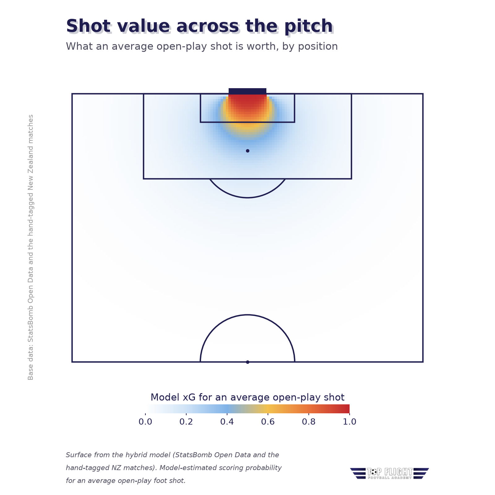 Figure 1: Shot value across the pitch
The hybrid model’s estimated scoring probability for an average open-play foot shot, by position. Value climbs steeply as chances move closer and more central, and falls to almost nothing beyond the box. Base data: StatsBomb Open Data and the hand-tagged New Zealand matches.
Two qualities matter when judging an xG model, ranking and calibration:
- Ranking asks whether the model places better chances above worse ones. A close-range chance should usually rate above a speculative shot from distance.
- Calibration asks whether the probabilities match outcomes across many shots. If a group of chances valued around 0.30 xG produces goals about 30% of the time, the model is well calibrated for that group. It is the harder property, and the one that breaks when a model trained on one standard of football is pointed at another.
The best-resourced models use more detail than this one, including information about defenders and goalkeepers at the moment of the shot. This model uses distance, angle, body part, rebound status and phase of play. That smaller set reflects what can be tagged consistently from local match video.
Those missing details can affect both the ranking and the probability of individual chances. The question tested here is whether adjusting a simpler model with local outcomes improves its overall calibration. It cannot replace the detail available to a model with freeze-frame data.
None of this is really about New Zealand. It is about the level. Full-time professionals train most days. National League players fit training around work or study, and so do the goalkeepers and defenders they face. Point an elite model at a French Regional 2 derby between USJA Carquefou and AC Basse-Goulaine and it would get the numbers wrong for the same reason. The shooter is sharper in the elite game, yes, but so is everything built to stop him. Which of those two truths wins out, and by how much, is the whole question, and the next section starts to answer it.
3 The data behind it
An xG model begins with the arduous, less glamorous task of recording the shots, one by one. Large datasets arrive with locations and outcomes already tagged. For this project, the only option was to build a local dataset from match footage, match by match.
Each shot was watched back and logged in Longomatch, a video-tagging tool, recording its location, outcome, body part and phase of play. Locations were marked by eye on a pitch scaled to 104 by 68 metres. A match typically yields 20 to 30 attempts. Rewinding footage helps, but hand-tagged positions remain estimates.
By the hundredth game, the full database held 2,514 shots from 100 matches across ten competitions and match types. Removing the pre-season friendlies leaves 2,345 shots from 90 matches across eight competitions. The model learns from the competitive fixtures only, meaning the Chatham Cup, the National League Championship and the upper regional leagues in the north and centre, which make up 48 of those matches. The other 42 are lower-grade games from NRF League One and the Northern Conference, left out of training because, as Section 6 shows, they appear to play differently close to goal.
A database of more than 2,000 hand-tagged shots is a substantial collection for this setting, but the model learns from the 1,046 unblocked, non-penalty shots in the 48 competitive matches within it, which is small by modelling standards. That is why the elite data serves as a starting point and why uncertainty matters throughout this article.
Figure 2 plots every shot from the 90 matches outside the pre-season friendlies. Attempts cluster in and around the penalty area, as expected. The typical open-play attempt comes from around eighteen metres, more than half from inside the box, and only a handful from beyond thirty. That is a useful check on the recorded locations, though it does not, by itself, prove that every position was tagged accurately.
Penalties are recorded at the penalty spot rather than estimated from the video. That keeps their location consistent, and the model assigns the same value to every penalty because it has no information about the taker or the goalkeeper.
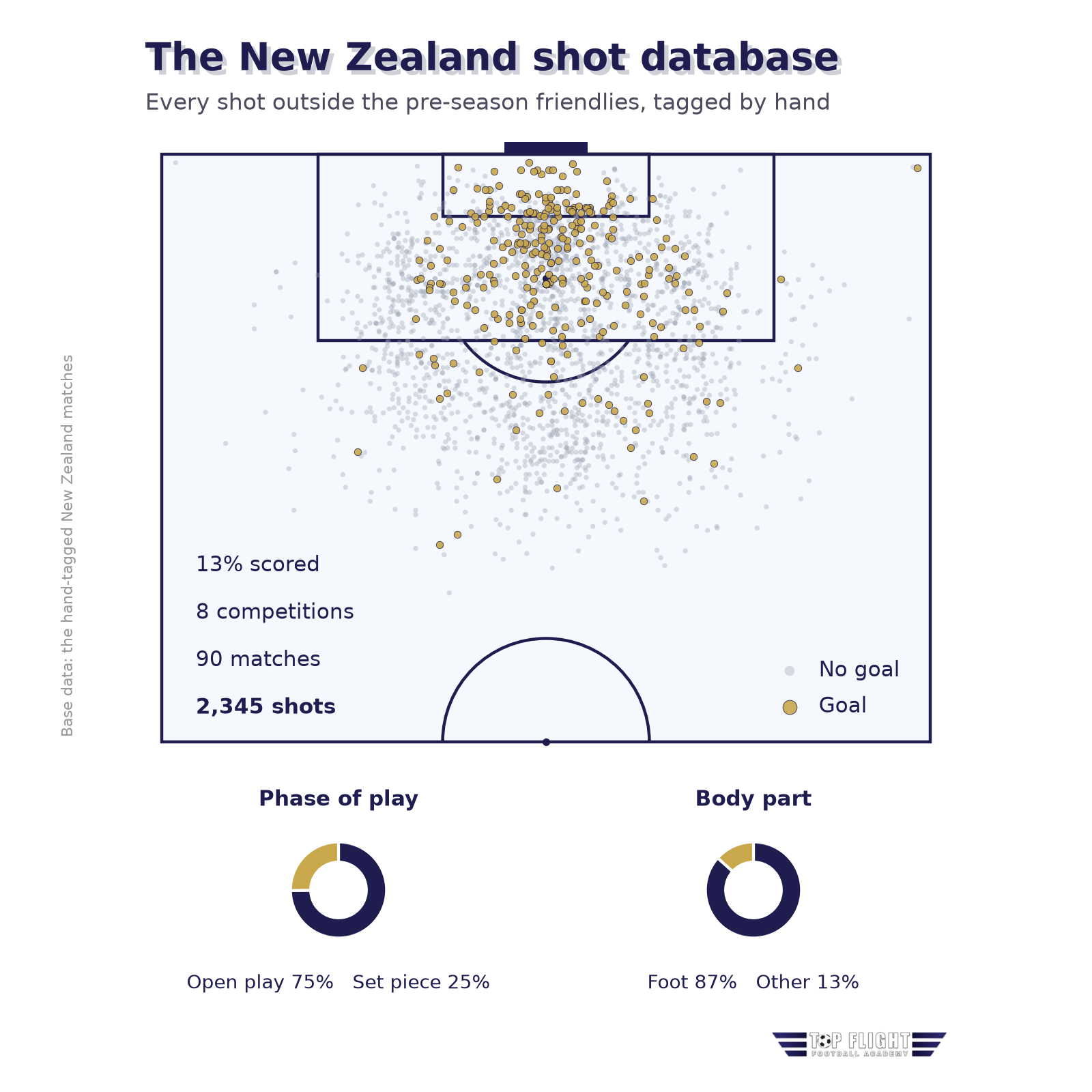 Figure 2: The New Zealand shot database
Every shot from the 90 matches outside the pre-season friendlies (2,345 shots across eight competitions), normalised to attack upward, with goals in gold. The cloud is dense in and around the box and thins quickly beyond it, the shape careful hand-tagging should produce. Below, the split by phase of play and by body part. Base data: the hand-tagged New Zealand matches.
4 Why neither dataset is enough on its own
Sections 1 and 2 left a question hanging. Point an elite model at New Zealand football and it will misprice a shot, but by how much, and in which direction? The answer is not the one most people guess.
Take a clean strike from the middle of the box. The intuition most people reach for is that a full‑time professional finishes it more often than a player at this level, so an elite model must be too generous for the local game. The numbers say the reverse. From that range, roughly one in six New Zealand open-play chances in this sample became goals, against closer to one in eight in the elite comparison, and beyond point-blank range local conversion was generally higher at similar distances. Distance alone does not make two chances identical, since angle and defensive pressure may still differ.
One likely explanation is that a shot is not just a striker but a striker against a goalkeeper and a defense, and at this level all of them are some way from the professional standard. The finishing may be less clinical, but weaker goalkeeping and slower defending could more than offset it. The data is consistent with that account without isolating the causes. Part of the gap could also come from the recording itself. One person tagging from video may log fewer speculative or hurried attempts than the event data behind the elite dataset, which would lift local conversion without any change in how the football is played. Blocked shots are left out of both datasets, so they do not explain it, but the data cannot rule out differences in what counts as a shot. What matters for the model is the observed result. An elite-trained model, which learned its rates against elite goalkeepers and defenders, tends to expect fewer of the local chances to go in than actually do. It does not flatter New Zealand shots. If anything it leans a little low, and Section 7 puts a size on that.
That is a level problem, and a borrowed model cannot fix it on its own. Its ranking is fine, since a good chance is still a good chance, but its numbers can come out low. So why not learn only from local shots? Their overall conversion rate reflects this sample, but only about a thousand competitive shots leave sparse examples for particular combinations of distance, angle, body part and phase of play. Ask a local-only model about a header from a tight angle and it is working from a handful of examples, so its estimate can move sharply when a few shots are added.
The two sources fail in opposite and complementary ways. The elite model has the shape right and the level wrong, while the local model has the level right and the shape wobbly. So each is used for what it does well. The elite data supplies the shape, how a chance decays with distance, what an angle costs and what a header gives up against a clean strike with the foot, and the local outcomes pull that surface to the level of the game played here. The technical name is domain adaptation, a close relative of what is often called transfer learning. In simpler terms, borrow the shape and correct the level.
Does it work? The test is the one Section 2 set out, not whether the model ranks shots but whether its numbers are true. Three models, one trained on elite data only, one on New Zealand shots only and the hybrid using both, were each shown the same 48 competitive New Zealand matches that none of them had trained on, and the question was how far their probabilities sat from what actually happened. That distance is called ‘calibration error’. Gather every chance a model called 0.20, and if twenty in a hundred were scored its error is nothing, while if thirty in a hundred were scored it was badly out. Averaged across every level of xG, that gives one measure of how truthful a model’s probabilities are, where lower is better. The measure, expected calibration error (ECE), depends on how probabilities are grouped, so it is read alongside its uncertainty and the goal totals. Figure 3 shows how the three models compared.
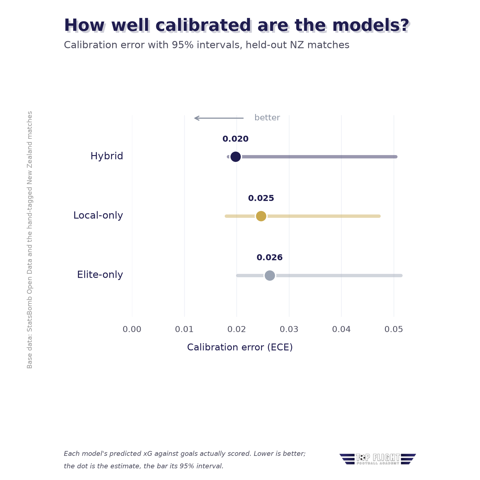
Figure 3: How well calibrated are the models?
Each model’s calibration error (ECE) on the same held-out New Zealand matches, with 95% intervals. Lower means the predicted xG sat closer to real goal rates. The hybrid ranks best, the local-only model next and the elite-only model last, though the intervals overlap, so on a 48-game sample the order is suggestive rather than settled. Base data: StatsBomb Open Data and the hand-tagged New Zealand matches.
The hybrid model came out best, in the sense that its calibration error was the lowest of the three, scored on every shot. In the point estimates, its stated xG sat closer to real New Zealand goal rates than either the elite-only or the local-only model’s, with those two close behind and effectively level. That is encouraging evidence for borrowing the shape and correcting the level.
The figure is honest about something else, though. Every estimate carries a band around it, the range the true error could plausibly fall in given only 48 held-out matches, and those bands overlap. The hybrid’s lead is real in the point estimate, and it points the way the argument says it should, but these matches do not establish a clear advantage over every alternative. None of this is a retreat from the finding. It is the honest state of the evidence, and the reason this article is pinned to a hundred-game milestone rather than a claim of proof. The result supports further development of the hybrid, and Section 7 returns to how hard those numbers can be pushed.
5 Letting the data set the dial
The last section made the case for blending elite and local data. The harder question underneath it is how much weight the local data should get, and for a long time that was a judgement call.
Think of the blend as a single dial. Turn it all the way one way and the model listens only to elite football, ignoring New Zealand entirely. Turn it all the way the other and it throws the elite data out and learns from local shots alone. Everywhere in between, the dial sets how loudly the New Zealand data gets to speak over the elite baseline. Turn it low, and the local games only nudge it; turn it high and they shout it down. The whole question is where to leave the dial.
An early version of this model set the dial by feel, weighting the local data heavily for no better reason than that it seemed about right. That is not good enough for a number meant to be trusted, so each setting was tested instead. For every setting, the model learned from part of the New Zealand dataset and was assessed on matches left out of that training split, and repeating this across splits shows how calibration changes as local data receives more weight. Figure 4 shows the results.
Pure elite had the highest error point estimate in the sweep, but the margin is small, because differences between settings are modest relative to the variation across folds. That fits the argument from Section 4, without proving it. Once any local data is let in, the settings are genuinely hard to tell apart, the line wandering through a wide band of uncertainty rather than dropping into a clean valley. The result favours including local evidence without identifying one precise weight. A hundred games is enough to suggest that local data helps. It is not yet enough to say precisely how much.
So the dial sits at 0.5, the lowest point in the sweep, a setting where the New Zealand data counts for about half its raw weight. A nearby setting might perform just as well on another set of matches. The nested cross-validation in Section 7 points the same way. Its five outer folds each chose the weight afresh and landed on 1.0, 0.1, 0.25, 0.5 and 2.0, so the preferred setting moves with the matches, which is what a flat basin looks like.
As the database grows, the choice can be tested again. More local shots may justify a different weight, but the direction of any change should be measured rather than assumed. At a hundred games the blend can be located to a broad region but not to a single figure, and the way to sharpen it is the same as ever, more matches.
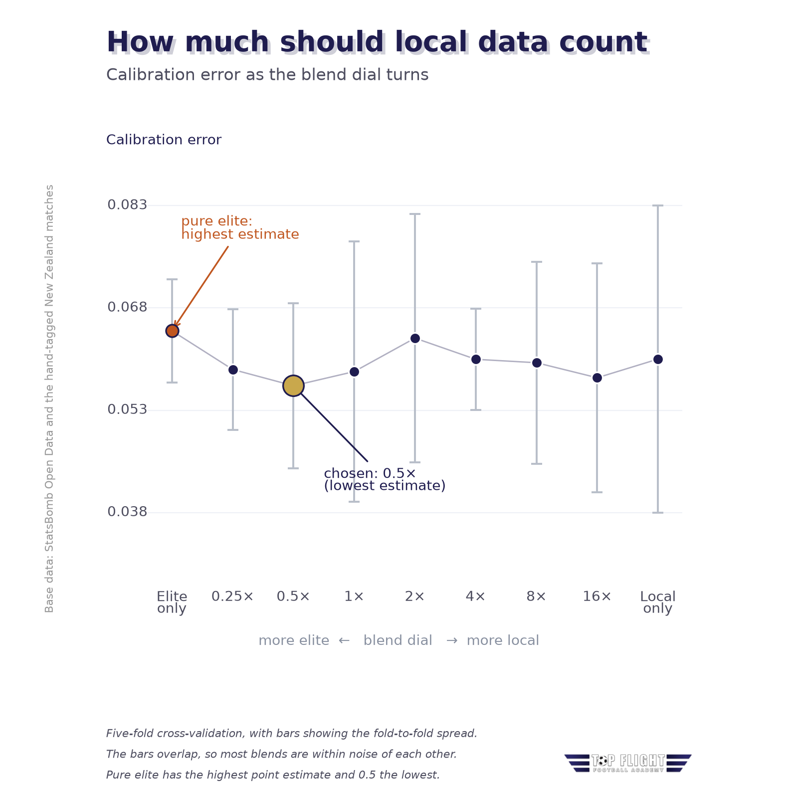
Figure 4: How much should local data count?
Calibration error on held-out New Zealand matches as the blend dial turns from pure elite (left) to pure local (right), from five-fold cross-validation. Bars show the fold-to-fold spread and overlap heavily, so most settings cannot be told apart with confidence. Pure elite has the highest point estimate and 0.5, the chosen setting, the lowest. Each fold holds only about eight matches, so the error here runs higher than the pooled error reported for the hybrid model, which scores all 48 held-out matches together. The curve is for comparing settings, not for reading off absolute error. Base data: StatsBomb Open Data and the hand-tagged New Zealand matches.
6 What the model learned from the shots
Three choices are especially useful for understanding the model, which levels of football to include, how to treat set pieces and which features to leave out.
The levels are not the same game. New Zealand’s domestic football is not one standard but several, stacked on top of each other from the National League down through the regional grades. The temptation is to pool them all for more data, but the shots suggest the levels play differently, at least close to goal. Take open-play chances from within 18 metres. Conversion is similar there, about 22% in the competitive grades and 25% in the lower grades. Within 11 metres the gap widens, with the competitive grades converting 32% against 41% in the lower grades. Figure 5 shows both bands. Neither gap is large against the number of shots behind it, so this is a hint rather than a finding. That close-range gap runs in the same direction as the one Section 4 found between the elite game and the local one, appearing again one rung further down. These shots are not perfectly matched for angle, defensive pressure or other context, so the gap cannot be put down to playing standard alone. The model is trained on competitive matches only, so it learns the conversion rates of the football it is meant to describe. When the lower-grade games were added back and tested under cross-validation, calibration did not measurably change, so this sample does not prove that leaving them out makes the model sharper. Training on competitive matches is the right call for describing competitive football, but it is not yet a call the data can force.
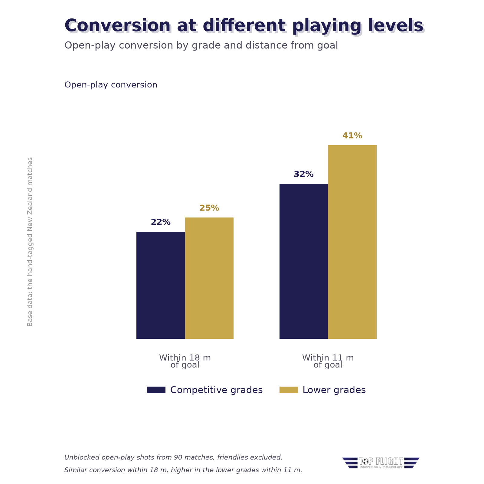
Figure 5: Conversion at different playing levels
Conversion of unblocked open-play shots in the 90 matches outside the pre-season friendlies, comparing competitive and lower grades within 18 m and within 11 m of goal. Conversion is similar within 18 m and higher in the lower grades within 11 m, though the gaps are small against the number of shots and other shot characteristics may also differ. Base data: the hand-tagged New Zealand matches.
Set pieces are their own species, and not in the way you might guess. A shot is never just a location, it is a location arrived at in a particular way, and the model prices that difference. Once distance and angle are accounted for, the phase of play still moves the number. The model gives corner shots a lower probability than open-play shots from the same spot, perhaps because a corner drops the ball into a crowded six-yard box. The raw conversion rate hides this, since corner shots come from close in and look ordinary, but they go in less often than that closeness should deliver. Direct free kicks run the other way. They are struck from distance, where geometry alone would price them very low, yet the model gives them a higher estimate than open-play attempts from comparable range. Indirect free kicks, once the geometry is handled, behave much like open play, and throw-ins are grouped with open play because a shot taken a few seconds after a throw is, by the time it is struck, just an open-play shot. Figure 6 shows the fitted coefficients, including body part and rebound status. These are associations learned from the available shots, not proof that one kind of delivery causes a particular outcome, and direct free kicks in particular are scarce in this sample, so their estimated effect is held more loosely than the distance and angle effects.
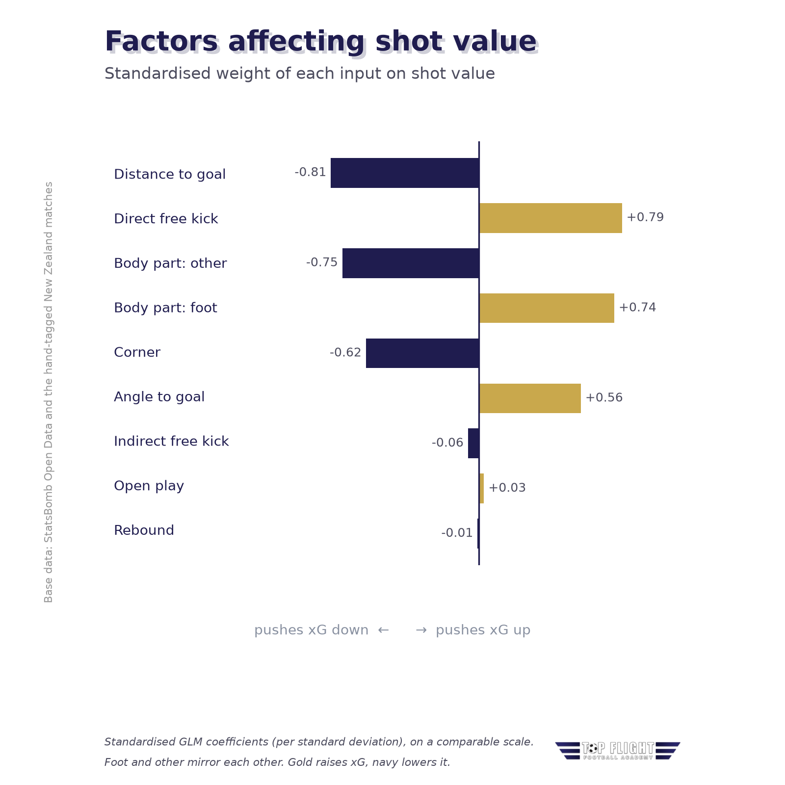
Figure 6: Factors affecting shot value
The fitted model’s standardised coefficients, which put distance, angle and shot type on a comparable scale. Distance has the largest effect, with value falling as shots move further out. Direct free kicks and a wider angle push the estimate up, and corners push it down. Foot and other body parts are two sides of one choice, so their bars mirror each other. Rebound, indirect free kicks and open play sit near zero. Gold indicates a higher predicted probability and navy a lower one. Coefficients describe model associations, not the independent causal effect of each factor. Base data: StatsBomb Open Data and the hand-tagged New Zealand matches.
What did not matter. One test asked whether telling the model which half of the match a shot came from would help, on the hunch that game state or tiring legs might shift how chances are finished. Alternative selections of the elite data and finer set-piece categories were tested the same way. None improved calibration measurably under cross-validation, so they were left out. That does not show they never matter, only that this sample did not support adding them. A null result, said plainly, is not a hole in the work. It is the difference between a model tuned on evidence and one tuned on hunches.
7 How did it perform on unseen matches?
The most useful test of a model is how it performs on matches left out of its training.
A model can always be made to look good by letting it see the games it is judged on, or by tuning its settings on the same data used to score it. To avoid both, the blend was chosen and scored with nested cross-validation. It works in two layers. An inner layer picks the settings, and an outer layer then tests the finished model on games neither layer has seen. Every number that follows comes from games the model never trained on, and every number is reported with the uncertainty around it.
Five models went into the same test. Three are the models from Section 4, elite-only, local-only and hybrid. The other two are reference points to keep them honest. The first is a field-standard model, the kind of open-play xG an analyst would build from distance, angle and body part on elite data alone, with no local calibration. It answers the obvious challenge of whether all this local work beats simply doing the normal thing. The second is a deliberately stripped-down version of the model, there to check that the features it uses earn their place. Both can price open play only, so for a fair comparison all five are scored on the same 814 open-play shots, out of the 1,046 held out. Figure 7 shows how they compared on calibration error.
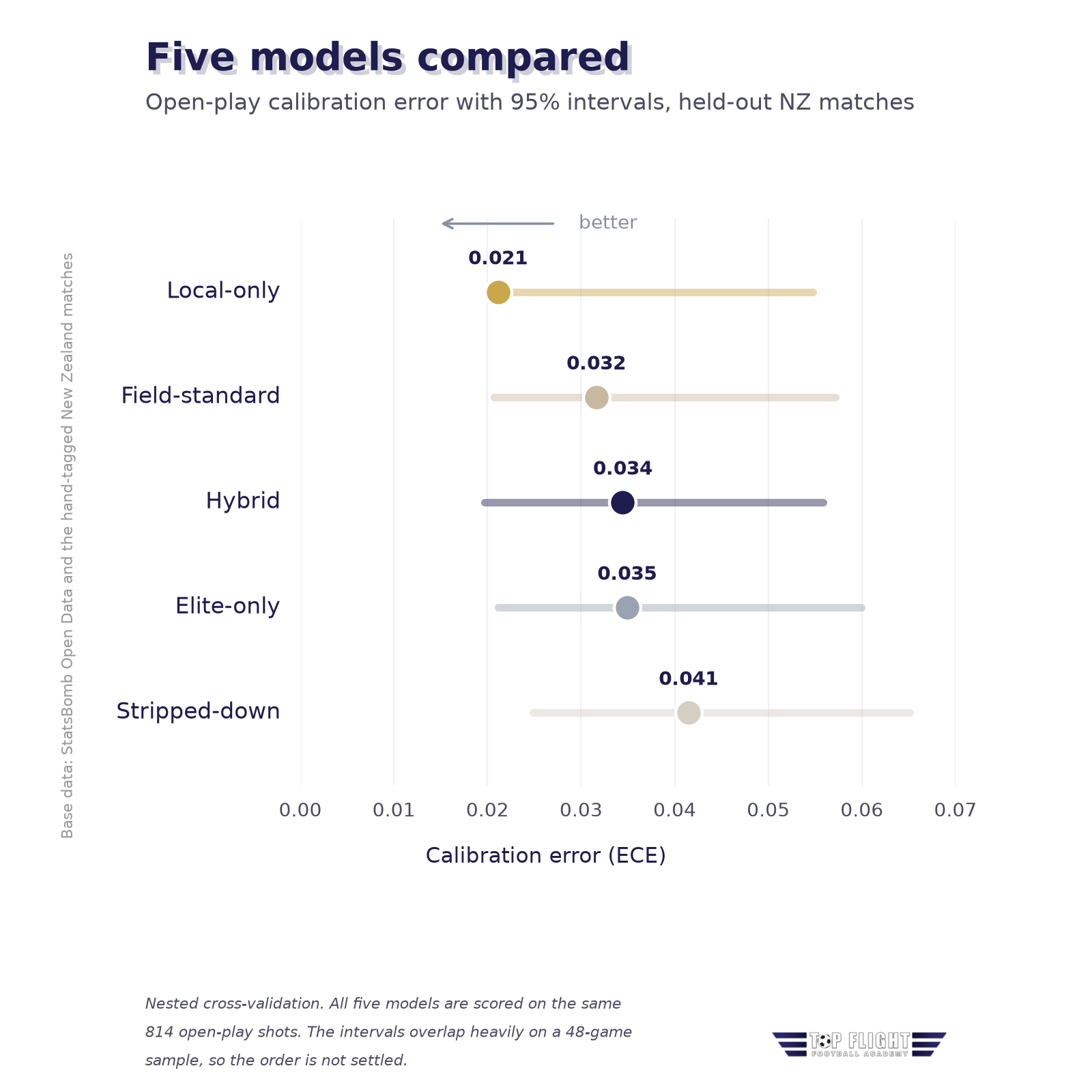
Figure 7: Five models compared
Each model’s calibration error (ECE) on the same 814 open-play shots from the held-out competitive matches, from nested cross-validation, with 95% intervals. The local-only model has the lowest point estimate, followed by the field-standard model, the hybrid, the elite-only model and the stripped-down control. The intervals overlap heavily, so on a 48-game sample the ordering is not settled. Base data: StatsBomb Open Data and the hand-tagged New Zealand matches.
On open play, the local-only model had the lowest calibration error, followed by the field-standard model, the hybrid, the elite-only model and the stripped-down control, but the gaps between them are small against the uncertainty. Scored on all 1,046 shots, as in Section 4, the hybrid has the lowest point estimate, so its position depends on whether set pieces are included. Paired comparisons over resampled matches are a sharper test than overlapping intervals, because every model is scored on the same games, and they did not separate the hybrid from any rival on calibration error. The one clear difference was in log loss, a measure that punishes confident wrong probabilities, where the hybrid beat the local-only model on all shots. That fits the argument that the elite data supplies useful shape which 48 matches cannot supply alone.
The totals give a second check. Across all 1,046 held-out shots, 158 goals were scored. The hybrid expected about 156, the local-only model about 158 and the elite-only model about 154. On open play, where all five can be compared, 125 goals were scored. The hybrid and local-only models expected about 124, the elite-only model about 122, and the field-standard and stripped-down models about 118. Every model fell short, the hybrid and local-only models by about one goal, the elite-only model by about three and the two reference models by about seven. That ordering fits the argument that elite-trained models run low, although the stripped-down model uses local data too, so the data source is not the whole story. The gaps are small against the interval around each total, which is wide, roughly twelve goals either way, so the totals show a lean rather than a measured error. Close totals are useful, although agreement in aggregate can hide errors on particular kinds of shot.
All of this rests on 48 competitive matches. That is a real sample, built up over five seasons, but a small one, and the uncertainty around every number is wide to match. The fair summary is that no model clearly wins on calibration. The hybrid is at or near the top on most measures and is the only model to clearly beat another, the local-only model on log loss, but a hundred games can only settle so much, and more matches will give a firmer test of whether its advantage holds.
The five models separate goals from non-goals about equally well, with their ability to rank one shot above another sitting between 0.77 and 0.79 for every one of them. The stripped-down control ranks slightly highest, despite being the worst calibrated of the five. Ranking and calibration answer different questions. A model can tell which chances are relatively good while attaching probabilities that are less reliable. Telling a good chance from a bad one was never the hard part. Saying how good, in numbers that come true for the football actually played here, is the part that took the work. Figure 8 sets each model’s expected goals against what was really scored.
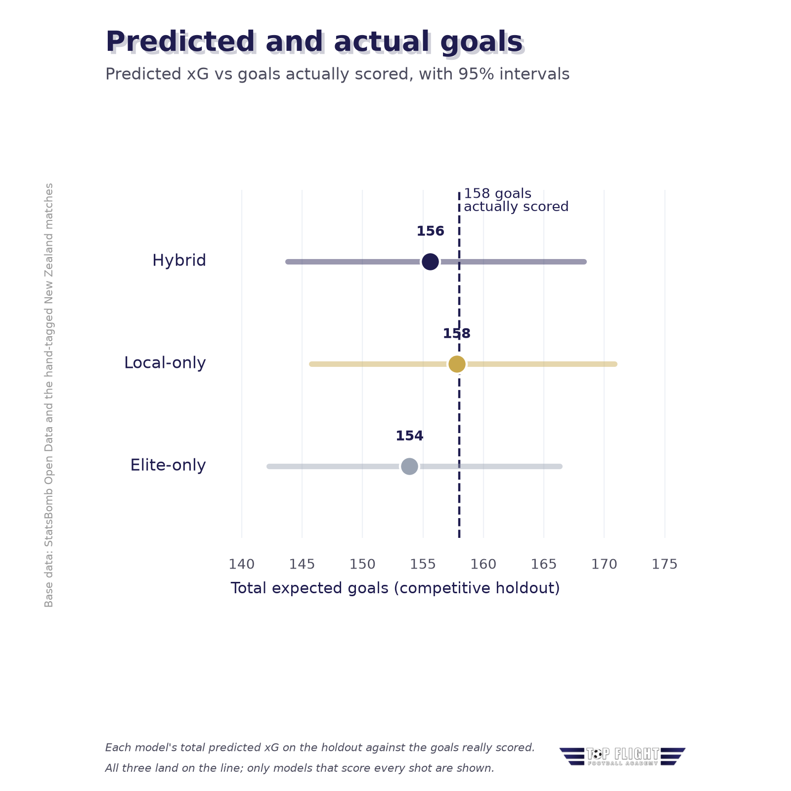
Figure 8: Predicted and actual goals
Total predicted xG from the models that price every shot, with 95% resampling intervals, against the 158 goals actually scored in the competitive holdout (dashed line). Open-play-only models are left out because their totals cover fewer shots. Base data: StatsBomb Open Data and the hand-tagged New Zealand matches.
8 What xG revealed about Petone’s season
The model can also help a coaching group ask better questions about a season. Across the 2026 season, every competitive Petone FC Men’s First Team match was tagged and run through the model, for and against, shot by shot. The tagging was done as part of the post-match xG reporting that the author (T. Billac) provides to Petone FC at the club’s request. What comes back is a second account of the season, one that sometimes agrees with the scoreline and sometimes disputes it.
One away match shows the difference between a result and its chances. Petone lost one-nil, yet the model had them creating 3.27 expected goals and conceding 0.84. That does not mean a win was guaranteed, but the chances favoured Petone far more strongly than the scoreline suggests. On another day that game is a comfortable win, and the only place that is written down is the shot data. It was chosen because the gap is so clear, and most matches are less dramatic.
One match on its own is only an anecdote, though. Across 21 matches, Petone created 30.5 expected goals and scored 19. They conceded 36.5 expected goals and let in 37. Most of these matches also sit in the database the model learned from, so this describes the season rather than testing the model on games it had not seen.
At the back, the goals conceded matched the chances allowed almost exactly, 37 against 36.5 expected. That says something precise and narrow. The team conceded about as many goals as the chances against them were worth, and nothing more. It does not say whether giving up 36.5 expected goals was acceptable, or whether particular goals involved preventable errors. At the other end, Petone scored about 11.5 fewer goals than the model expected from their shots. This is a sizeable gap, and it should not be heard as a dig at the players taking the shots. Expected goals alone cannot separate finishing skill from chance details the model missed or ordinary variation across a season.
Petone’s expected goal difference across the 21 matches was minus six, while their actual goal difference was minus 18. On the balance of chances they were a little below their opponents, which is a modest gap, and almost all of the twelve goals between the two figures comes from the scoring end. That is a useful prompt for reviewing the shots and the attacking process, not a verdict on individual players.
For the coaching group, the next step is to watch those chances again. Which attempts were repeatable, what pressure were the shooters under, and where might a simpler model have missed important context? Shot volume against shot quality is a natural place to start, because 30.5 expected goals can come from many modest chances or a few good ones, and the two call for different fixes. Figure 9 shows the away loss as one example of the season-wide gap.
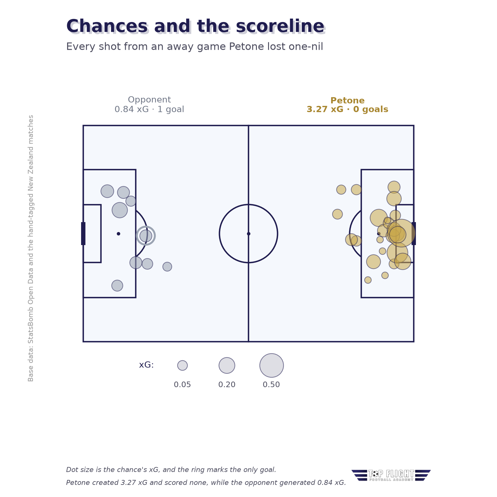
Figure 9: Chances and the scoreline
Every shot from an away game Petone lost one-nil, sized by xG, with the only goal ringed. Petone created 3.27 expected goals and scored none, while the opposition generated 0.84 and scored once. Base data: StatsBomb Open Data and the hand-tagged New Zealand matches.
9 What the next hundred matches could teach us
The model is already useful for asking questions about matches, and the next hundred games should give a firmer test of its probabilities.
Its shot values feed match reports, season summaries like the one in Section 8, and an early dashboard for coaches. Those outputs matter most when they lead back to video and a discussion of the chances behind the numbers.
A larger local sample could help test additional details, such as whether a shot was taken first time and how set-piece sequences developed. It should also narrow the uncertainty around the blend weight and the model comparisons. Each new feature should earn its place on the evidence rather than a hunch. Much of what is still uncertain has the same remedy, which is more matches.
Other limitations need different solutions. One person tagged the local shots, so independent checks of location and classification would strengthen confidence in the data, including whether every attempt a professional provider would count as a shot has been logged. Without freeze-frame information, the model cannot see where defenders stood or how the goalkeeper was set. Those limits should stay visible whenever its estimates are used.
To the authors’ knowledge, there was no openly available expected-goals model for New Zealand football. After a hundred tagged matches, there is now a working one. The hybrid had the lowest calibration error of the three models scored on every shot and was clearly better than the local-only model on log loss, but no model separated cleanly on calibration error, so the size of any advantage remains uncertain. The next hundred matches can test whether it holds.
If your club would like to contribute match footage and explore what the model says about your chances, get in touch through the contact page on this site, on X at @TOFFA2023 or on Instagram at @the_toffa_analyst. Come and be part of the second hundred.